Data Mining with R or Python

What is data mining? There are various ways to go about the process. Let’s dive into data mining techniques with R and Python.

Data Mining: Mining in the 21st Century

Data mining is the mining technique of the 21st century. But what is it exactly? We’ll define the meaning of ‘mining’ first. 

Mining is extracting valuable minerals or other materials like coal from a mine or placer deposit. Similarly, data mining is extracting potential information and insights from big data. 

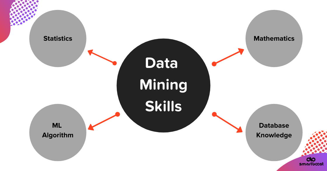
Data mining uses statistics, mathematics, machine learning algorithms, database knowledge, and AI to analyze and extract insights and predict future events. The insights derived from data mining apply to various fields like marketing, banking, credit fraud detection, and health care services.

Data mining plays a critical role in the day-to-day activities of a data scientist or machine learning engineer. It is a step by step procedure to be implemented. Miners can use various techniques like regression, classification, clustering. Next, we will discuss the implementation process and mining techniques.

Data Mining Implementation Process

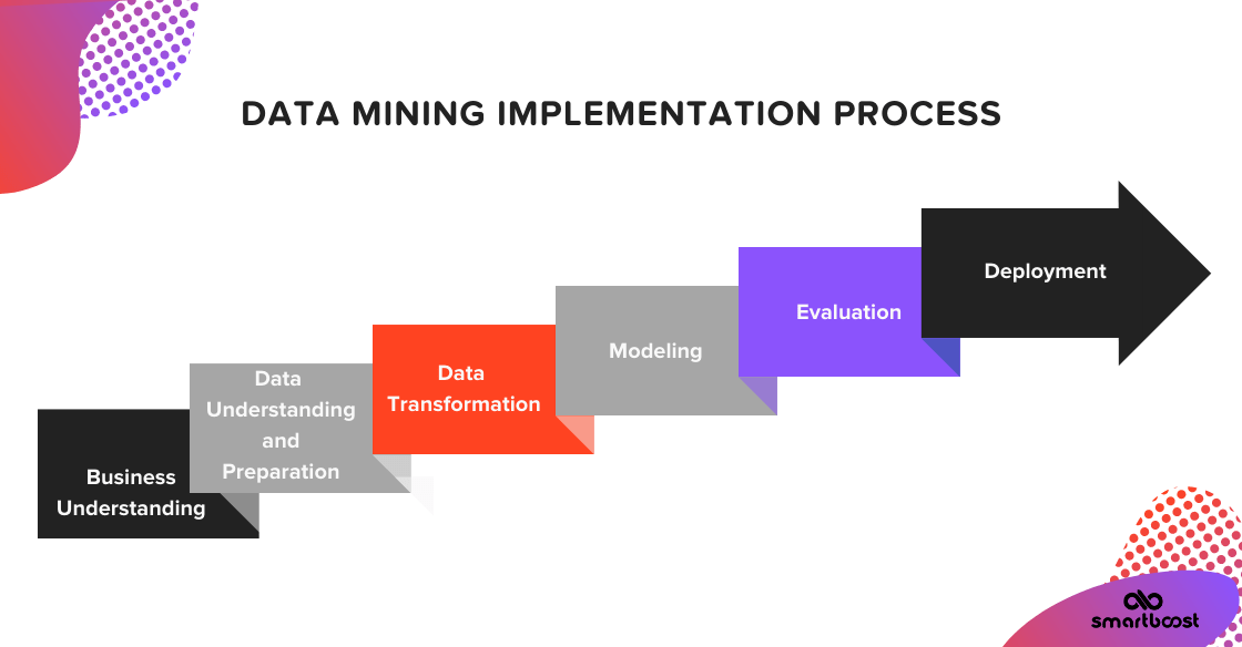
The data mining implementation process consists of 6 steps. Let’s discuss the whole process in detail.

Business Understanding

Before getting your hands dirty with data, the main job is to understand business objectives and the client’s perspective. Ask the questions below first:

• What are the client’s objectives and expectations?
• What are the business requirements that need to be met?
• What are the various resources available, different assumptions, and constraints?
• Have you prepared a good data mining goal and approach plan in detail?

Data Understanding and Preparation

After defining data mining goals, you’ll need to understand the data and prepare to mine. This activity consumes 90% of your time. The following steps are:

• Data collection from various sources.
• Merging of all data in a single format.
• Data needs to be cleaned and formatted.
• Removal of noisy data.
• Handling of missing data.
• Data outliers need to be taken care of at this step.

Data Transformation

Data transformation is crucial after this process. Miners use transformed data for modeling. Transformation techniques include:

Normalization

Data miners will use normalization to bring all the features on the same scale. This scaling technique will shift and rescale all features and get their values between 0 and 1.

Standardization

Standardization puts different variables on the same scale. To standardize a variable, you will need to calculate the mean and the standard deviation of said variable. Next, subtract the mean and divide by the standard deviation.

Feature Engineering

Feature engineering is crucial for accurate results of ML modeling. New features are created to ensure the algorithm works for the best based on domain knowledge and experience.

One-Hot Encoding

Many algorithms don’t work on categorical data or textual data. So, to convert categorical data to numerical data, use one-hot encoding.

Modeling

Complete modeling using a prepared dataset and various data mining techniques. Data modeling is a process to find a relationship between the input features and their relation to the output feature. The method of modeling includes:

• Selecting the appropriate ML algorithm according to the data-set and expected output.
• Training an ML model on training data using the ML algorithm.
• Meeting the data mining objectives as per the business.

Evaluation

At this stage, appropriate parties will evaluate the model. Complete the evaluation as follows:

• Evaluate the model according to the business objectives and requirements.
• Verify results against test data.
• Decide whether the model will go to the deployment stage or not.

Deployment

In this phase, deploy the data mining model to business operations. Keep the following in mind:

• We create data mining models to add value to the business only when deployed to its environment.
• Even non-technical people can easily use deployed models for the predictions of future events.

Data Mining Tools

Two tools for data mining are Python and R.

Python is a widely-used programming language that helps a programmer to work quickly and effectively. Python is in great demand for Machine Learning Algorithms. Many feature libraries like NumPy, pandas, SciPy, Scikit-Learn, Matplotlib, Tensorflow, Keras makes machine learning task very easy to implement with Python.

R is another tool that is popular for data mining. R is an open-source programming tool developed by Bell Laboratories (formerly AT&T, now Lucent Technologies). Data scientists, machine learning engineers, and statisticians for statistical computing, analytics, and machine learning tasks prefer R. R libraries like Dplyr, Caret, Ggplot2, Shiny, and data.table is used in machine learning and data mining.

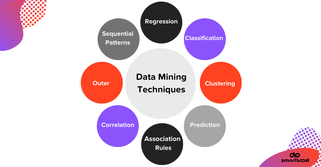
Data Mining Techniques

Eight data mining techniques are used extensively. We will discuss these techniques in detail with Python and R code snippets.

Regression

Regression is a data mining technique used to find the relationship between two or more variables. All the variables need to be continuous. Regression is a supervised learning technique of data mining used to predict the value of a dependent variable(Y) based on other independent variables(X’s). 

When a single independent variable is used to predict a dependent variable’s value, it’s called simple linear regression. In cases where two or more independent variables indicate a dependent variable’s value, it’s called multiple linear regression.

The best fit straight line is called a regression line. Linear regression is represented by the equation Y=b*X + a + e, where a is the intercept, b is the slope of the line, and e is the error term.

Python Code:

Let’s implement linear regression in Python on a Boston house-prices dataset to determine housing prices at various Boston locations for 13 features of the dataset.  We will create a linear regression model on train data first and then complete the test data prediction.

#Import Libraries from sklearn.datasets import load_boston from sklearn.model_selection import train_test_split from sklearn.linear_model import LinearRegression import seaborn as sns #Load data X = load_boston().data Y = load_boston().target # Split data train_x, test_x, train_y, test_y=train_test_split(X, Y, test_size=0.33, random_state=5)#Implementing Linear Regression lin_reg = LinearRegression(normalize=True) lin_reg.fit(train_x,train_y) pred = lin_reg.predict(test_x) sns.regplot(test_y, pred); plt.xlabel(‘Test Y’) plt.ylabel(‘Predicted Y’) plt.title(“Plot between Predicted and Actual target values”) plt.show()

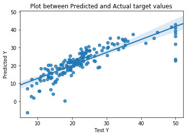The graph to the right shows the relationship between actual target values and predicted target values. The best-fit regression line is drawn to show the difference between the actual and predicted value and is used to find regression loss.

R Code

Let’s implement linear regression in R on a Boston housing-price dataset to determine housing prices at various Boston locations for 13 features of the dataset. Create the linear regression model on the train data using R, and then predict the test data.

#Load libraries library(MASS) #for loading dataset library(ggplot2) #for visualisation library(caTools) #for splitting data into testing and training data#Load Data housing<- Boston#Split data split <- sample.split(housing,SplitRatio = 0.75) train <- subset(housing,split==TRUE) test <- subset(housing,split==FALSE)#Implementing Linear Regression lm.fit1 <- lm(medv~.,data=train) test$predicted.medv <- predict(lm.fit1,test) ggplot(aes(x = medv, y = predicted.medv), data = test) +   geom_point(alpha = 0.5, color = ‘blue’)+   scale_y_continuous(‘y’)+   scale_x_continuous(‘x’)+   geom_smooth(stat = ‘smooth’, color = ‘Red’, method = ‘gam’)+   ggtitle(“Linear Regression”)

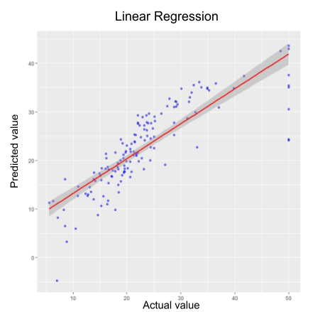
The graph to the left shows the relationship between actual target values and predicted target values. The best-fit regression line is drawn to show the difference between the two values and help find regression loss.

Classification

Classification is also a supervised learning technique used to classify input items in different classes. In the classification technique, the output variable (Y) is categorical.

Classification is like classifying dogs and cats’ images. It predicts which picture belongs to class ‘cat’ and which photo belongs to class ‘dog.’

Classification can be of two types: Binary classification has two output classes, and multi-class classification has multiple output classes.

Python Code:

Let’s implement logistic regression (a machine learning algorithm for classification) on Iris Dataset in Python. It is a flower dataset that has three output classes: setosa, versicolour, and virginica. 

Implement the logistic regression model on train data. Then, prediction will be done on test data. We will also draw a Confusion Matrix for performance analyses between actual and predicted values.

#Import Libraries from sklearn.model_selection import train_test_split from sklearn.linear_model import LogisticRegression from sklearn.metrics import confusion_matrixfrom sklearn.datasets import load_iris#load dataX = load_iris().dataY = load_iris().target#Split data train_x, test_x, train_y, test_y=train_test_split(X, Y, test_size=0.33, random_state=5) #Apply Logistic Regression Modeling log_model = LogisticRegression() log_model.fit(train_x, train_y) #Calculate Confusion Matrix pred=log_model.predict(test_x) df_cm = pd.DataFrame(confusion_matrix(test_y,pred),  range(3),range(3))    sns.heatmap(df_cm, annot=True, cmap=‘YlGn’, annot_kws={“size”: 20},fmt=‘g’)# font size plt.title(“Confusion Matrix”) plt.xlabel(“Predicted Label”) plt.ylabel(“True Label”) plt.show()

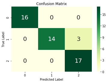
The image to the right shows a confusion matrix drawn for logistic regression. The confusion matrix is a performance analysis metric that defines the algorithm’s ability to predict the output classes accurately. 

We can see from the above Confusion matrix, out of 50 (= 16+14+3+17) test values, three are not predicted correctly, and 47 are predicted correctly. We can get the model accuracy = 47/50  = 0.94

R Code:

Let’s implement a decision tree classifier (a machine learning algorithm for classification) on Iris Dataset in R. It is a flower dataset with three output classes: setosa, versicolour, virginica. We will do modeling, prediction, and performance analysis using the confusion matrix for the dataset.

#Load libraries library(rpart) library(caret) #Split iris data dt = (sample(nrow(iris), 100)) train<-iris[dt,] test<-iris[-dt,] #Implement Decision tree Classification decision_tree_model<-rpart(Species ~ ., data = train, method = “class” Predicted<-predict(decision_tree_model,newdata=test,type=“class”) #Draw Confusion Matrix confusionMatrix(Predicted, test$Species)

The above image shows a confusion matrix drawn for the decision tree classifier. 

We can see from the above Confusion matrix, out of 50 (= 14+19+7+10) test values, 7 are not predicted correctly, and 43 are predicted correctly. Model accuracy = 43/50  = 0.86. 

Clustering

Clustering is an unsupervised learning technique. The technique’s use is to classify or cluster similar kinds of data from the dataset. In clustering, output class or value is not predicted.

Use clustering to group similar products, customers, and businesses.

Python Code:

Let’s implement k-means++ clustering (a machine learning algorithm for clustering) on Iris Dataset in Python. We will also draw a clustering graph of different clusters.

#Importing Libraries from sklearn.cluster import KMeans   #Applying kmeans to the dataset / Creating the kmeans classifier kmeans = KMeans(n_clusters = 3, init = ‘k-means++’, max_iter = 300, n_init = 10, random_state = 0) y_kmeans = kmeans.fit_predict(train_x)   #Visualising the clusters plt.scatter(train_x.iloc[y_kmeans == 0, 0], train_x.iloc[y_kmeans == 0, 1], s = 100, c = ‘red’, label = ‘setosa’) plt.scatter(train_x.iloc[y_kmeans == 1, 0], train_x.iloc[y_kmeans == 1, 1], s = 100, c = ‘blue’, label = ‘versicolour’) plt.scatter(train_x.iloc[y_kmeans == 2, 0], train_x.iloc[y_kmeans == 2, 1], s = 100, c = ‘green’, label = ‘virginica’) #Plotting the centroids of the clusters plt.scatter(kmeans.cluster_centers_[:, 0], kmeans.cluster_centers_[:,1], s = 100, c = ‘yellow’, label = ‘Centroids’) plt.title(‘Clustering graph’) plt.legend()

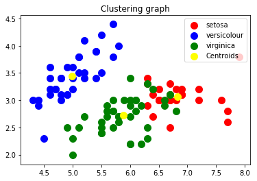
The graph to the left shows the dataset divided into 3 clusters; setosa, versicolour, and virginica, with their centroids. Three groups are easily distinguished using the clustering technique. 

R Code:

Let’s implement k-means clustering on the Iris dataset in R. We will also draw a clustering graph of different clusters.

#load libraries library(ggplot2) #kmeans clustering irisCluster <- kmeans(iris[, 3:4], 3, nstart = 20) table(irisCluster$cluster, iris$Species) #Clustering Graph plot_clusters<-ggplot(iris, aes(Petal.Length, Petal.Width, color = cluster)) + geom_point() plot_clusters

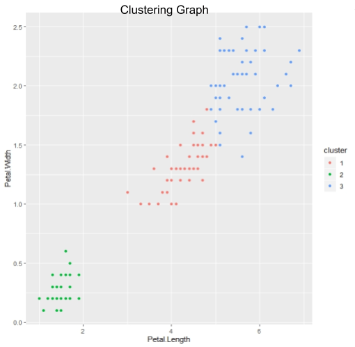
In the graph to the right, the dataset is divided into three clusters setosa, versicolour, virginica with their centroids. Three clusters are easily distinguished using the clustering technique. 

Prediction

We have learned different techniques of data mining like regression and classification. When a machine learning model is created, values are predicted on test data. 

Prediction is a fantastic data mining technique used to predict trends, patterns, forecasting, values, and classes. Past data or train data is analyzed and modeled correctly to predict future events.

Let’s implement Python code for logistic regression. In Python, predict values for test_x, and compare actual and predicted values using a scatter plot.

#load data X = load_iris().data Y = load_iris().target #Split data train_x, test_x, train_y, test_y=train_test_split(X, Y, test_size=0.33, random_state=5) #Apply Logistic Regression Modeling log_model = LogisticRegression() log_model.fit(train_x, train_y) #Calculate Confusion Matrix pred=log_model.predict(test_x)#Draw scatter plot for actual and predicted valuesplt.scatter(x=test_x[‘Sepal Length’], y=test_y,  label=’actual value’) ;plt.scatter(x=test_x[‘Sepal Length’], y=pred ,s=10, c=’r’, marker=”o”, label=’predicted value’) ;plt.title(“Scatter plot of Actual and Predicted Value”)plt.legend(loc=’upper right’);plt.show()

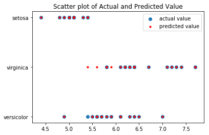
We can see actual values as a blue dot and predicted values as a red dot in the above scatter plot. It can be easily observed, except from 3 values, that the miner predicted all other data points correctly.

Association Rules

Association rule mining is a classical data mining technique used to identify interesting patterns in data. Association rule mining is used only for categorical data and is not suitable for numeric data. 

‘An association rule is a pattern that states that when X occurs, Y occurs with a certain probability.’

Association rules determined the relationship or association between two items. E.g., how frequently we brought two things like bread and milk together or milk and chocolates together. A man who went to bought ‘milk’ is likely to buy ‘chocolates,’ so stores placed them close to each other to increase sales.

Outer

Data mining’s outer technique is related to identifying data-set data, which behaves not as expected. Some data points might be noise points or some fraud data points. Detection of such data is known as outlier analysis or outlier mining. 

The outlier is a data point that lies outside or diverges too much from the rest of the dataset. In other words, we can say an outlier is a data whose value is much smaller or much more extensive than different values in the dataset.

The real-world datasets are not noise-free. They consist of outliers. Outlier detection is valuable in numerous fields like credit or debit card fraud detection, detecting network interruption identification, etc.

Let’s try to find some outliers in the Iris dataset using Python code.

import seaborn as sns sns.boxplot(x=‘Species’,y=‘Sepal Length’, data=data) plt.title(‘Boxplot of Sepal Length for 3 Species’) plt.show()

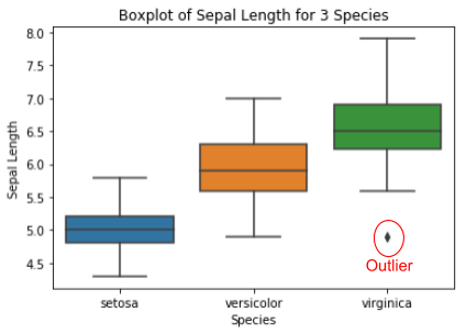
In the boxplot on the right, we can observe that in the Iris dataset, Virginica data-point have outlier(Point market in red). Outliers are points that fall outside the box-plot. Finding outliers from the dataset and pre-processing them is a fundamental data mining technique.

Sequential Patterns

The sequential patterns for data mining are specialized for periodicity analysis for sequence data. In real-world data, there are a considerable number of sequential patterns hidden. Mining techniques help to find them and analyze them.

There are many sequential pattern mining applications like music notes sequence, DNA sequence and gene structure, telephone calling patterns, or shopping experience.

Let’s understand with an example: A lady buys an expensive red color dress some days before Christmas. Then most likely, she will purchase matching footwear, purse, accessories, etc., in sequence. Predicting this shopping sequence is sequential pattern data mining.

Correlation

Correlation is a data mining technique used to define the relationship between two variables. Commonly used measurements are Pearson Correlation, Jaccob Similarity, Cosine Similarity, and Distance Correlation. We can determine the correlation between variables using a correlation coefficient. 

Statisticians typically write the correlation coefficient with R. The correlation coefficient value lies between 1 and -1. However, the closer R is to +1 or -1; the more closely the two variables are related. 

The closer R is to 0, the weaker the linear relationship. Positive R values indicate a positive correlation, where the values of both variables tend to increase together. Negative R values indicate a negative correlation, where one variable’s values tend to increase when the values of the other variable decrease. 

Let’s see the correlation between 4 features of the Iris dataset using Python code.

sns.heatmap(X.corr(),annot=True,cmap=“YlGnBu”)

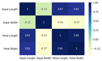In the heatmap on the left, we can observe that petal length and petal width are highly positively correlated with a coefficient value of 0.96. petal length and sepal width are negatively correlated with the coefficient value of -0.43. Similarly, we can extract the correlation between other features too.

Data Mining Applications

Data mining is beneficial in various domains. Let’s review some applications below:

• Banking: Data mining helps detect fraud cases in the credit card industry, fraud profiling, and fraud investment cases in banks.
• Manufacturing: With mining, it is easy to predict products that should increase or reduce their manufacturing based on market data.
• Insurance: Data mining helps insurance companies optimize the price of their most profitable products and predict which offers to promote to different types of customers.
• E-commerce: E-commerce sites, products price, product recommendations, and offers are all possible because of data mining.
• Education: Data mining can detect learning patterns in students using their background and achievement records to indicate who needs more attention and who should focus on a particular field.
• Service Providers: Data mining can be used in areas of the service industry like billing analyses, customer interaction, handling complaints, and detecting fraud in businesses.

Takeaway

Data mining is all about learning past data and predict the future.  Following the data mining implementation process with the various mining techniques, you can quickly discover, analyze, and forecast data. 

This article is not just for reading but also for implementing and practicing. Get your hands dirty and try data mining with Python or R, any language of your choice. Have fun with your data and its mining.